An example

The probability that a person will develop an infection even after taking a vaccine that was supposed to prevent the infection is 0.03. In a random sample of 200 people in a community who got the vaccine, what is the probability that six or fewer people will be infected?

sum(dbinom(0:6, 200, .03))

## [1] 0.6063152

pbinom(6, 200, .03)

## [1] 0.6063152

Poisson approximation to the binomial distribution

To use Poisson approximation to the binomial probabilities, we consider that the random variable \(X\) follows a Poisson distribution with rate \(\lambda = np = (200)(0.03) = 6.\) Now, we can calculate the probability of having six or fewer infections as

\[ P(X < 6) = \sum_{k=0}^{6}\frac{e^{-6} 6^k}{k!} = 0.6063 \] which turns out to be the same as we obtained with the binomial distribution.

We can verify the calculation in R

ppois(6, lambda = 6)

## [1] 0.6063028

Clearly, Poisson approximation is very close to the exact probability.

Normal approximation to the binomial distribution

We can also calculate the probability using normal approximation to the binomial probabilities. Since binomial distribution is for a discrete random variable and normal distribution is for continuous random variable, we have to make continuity correction to approximate a binomial distribution using the normal distribution.

For large \(n\) and when \(np > 5\) and \(nq > 5,\) a binomial random variable \(X\) with \(X \sim Bin(n, p)\) can be approximated by a normal distribution with mean = \(np\) and variance = \(npq.\) That is, \(X \sim N(6, \, 5.82).\)

Therefore, the probability that there will be six or fewer cases of incidences can be calculated as

\[ P(X \leq 6) = P\left(z \leq \frac{X-6}{\sqrt{5.82}} \right). \] As mentioned earlier, we have to make the continuity correction, and so the above expression will become \[ \begin{align*} P(X \leq 6) &= P\left(z \leq \frac{(X+0.5) - 6}{\sqrt{5.82}} \right) \\ &= P\left(z \leq \frac{6.5-6}{\sqrt{5.82}}\right) \\ &= P(z \leq 0.2072) \end{align*} \]

Using a standard normal table or using R, we can obtain the probability, which is 0.5821

pnorm(.2072)

## [1] 0.5820732

We note that the approximation is close to the exact probability 0.6063 but the Poisson approximation does much better.

Simulation

To see how the good the approximations are in repeated samples, we generate 1000 random sample of size 200 from a normal distribution with mean = 6 and standard wwwiation = 5.82. The generated data are used to approximate the binomial probability using Poison and normal distributions.

We use the following code to generate the figure below.

apprx <- function(n, p, R = 1000, k = 6) {
     q = 1- p
     trueval <- pbinom(k, n, p) # true binomial probability
     prob.zcc <- prob.zncc <- prob.pois <- NULL  
     for (i in 1:R) {
          x <- rnorm(n, n * p, sqrt(n * p * q))
          z.cc <- ((k + .5) - mean(x))/sd(x) # with cont. correction
          prob.zcc[i] <- pnorm(z.cc)
          z.ncc <- (k - mean(x))/sd(x) # no cont. correction
          prob.zncc[i] <- pnorm(z.ncc)    
          y <- rpois(n, n * p)
          prob.pois[i] <- length(y[y <= k])/n
     }
     list(prob.zcc = prob.zcc, prob.zncc = prob.zncc, 
          prob.pois = prob.pois, trueval = trueval)
}

R <- 1000
set.seed(10)
out <- apprx(n = 200, p = .03, k = 6, R = 1000)
# windows(6,5)
plot(1:R, out$prob.pois, type = "l", col = "green", xlab = "Runs", 
     main = expression(paste("Simulated Probabilities: ", 
                             n==200, ", ", p==0.03, sep="")),
     ylab = "Probability", ylim = c(.3, .7))
abline(h = out$trueval, col="red", lty=2)
lines(1:R, out$prob.zcc, lty = 1, col = "purple")
lines(1:R, out$prob.zncc, lty = 1, col = "orange")
legend("bottomleft", c("Poisson", "Normal (with cc)", 
                       "Normal (w/o cc)"),
       lty = c(1), col = c("green", "purple", "orange"))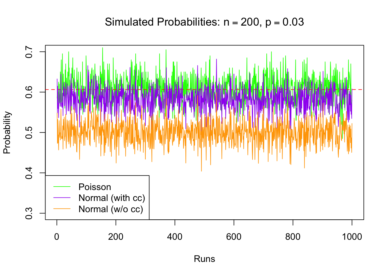

Above figure shows the calculated probabilities for each run of the simulation. The read horizontal line at 0.6 shows the exact probability. The figure shows that the normal approximation, with or without continuity correction, is underestimating the exact probability while Poisson does a better job approximating it for \(n=200\) and \(p=0.03.\)

Since this plot does not reveal much due to overlapping points, we draw boxplots for the calculated probabilities for \(n= 100, 200, 233, 300,\) and \(p=0.03.\)

# n = 200
set.seed(10)
out <- apprx(n = 200, p = .03, k = 6, R = 1000)
# windows(6,5)
boxplot(out$prob.pois, boxwex = 0.25, at = 1:1 - .25,
        col = "green",
        main = expression(paste("Approximating Binomial Probability: ", 
                                n==200, ", ", p==0.03, sep="")),
        ylab = "Probablity", 
        ylim = c(out$trueval - 0.2, out$trueval + 0.25))
boxplot(out$prob.zcc, boxwex = 0.25, at = 1:1 + 0, add = T,
        col = "purple")
boxplot(out$prob.zncc, boxwex = 0.25, at = 1:1 + 0.25, add = T,
        col = "orange" )
abline(h = out$trueval, col = "red", lty=2)
legend("topleft", c("Poisson", "Normal (with cc)", "Normal (w/o cc)"), 
       fill = c("green", "purple", "orange"))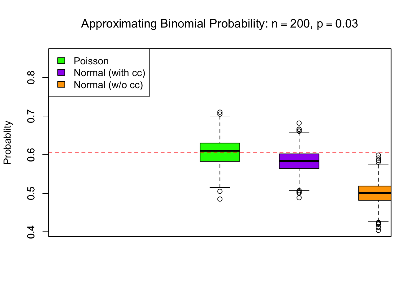

Conclusion

To summarize, we see that for \(n = 200\) and \(p = 0.03,\) Poisson does better than the normal with continuity correction. However, for larger sample sizes, especially when n is close to 300, the normal approximation is as good as the Poisson approximation. It is to be mentioned here that the normal based approximation has always narrower spread than the Poisson based approximation. More importantly, the results are true for this particular case when \(p=0.03.\)